

With the oldest baby boomers over eleven years into retirement and the oldest Generation X members just eight years away, we now have over 135 million people in the U.S. actively planning for retirement or already living off their savings. According to the distribution of household wealth maintained by the Federal Reserve1, these two generations comprise over 82% of all corporate equities and mutual fund investments. Bond returns for the youngest individuals in this cohort have averaged 6.75% per year from 1980 through 20222, helped by a large tailwind from falling interest rates. The overlap of large numbers of individuals planning for retirement and the strong returns of bonds has led to the popularity of investment strategies such as “age-in-bonds” and “target date funds,” which encourage an increased allocation to bonds as the investor ages. Morningstar3 estimated that over $2.82 trillion was invested in target-date funds at the end of 2022. The gradual reduction in exposure to stocks as retirement nears results from a narrow focus on volatility as the primary relevant measure of portfolio risk. With lower yields causing bond returns to fall to just over 2% on average from 2009 through 2022, the risk of running out of money during retirement significantly increased for investors in these strategies.
Furthermore, the length of an investor’s planning horizon contributes to “longevity risk,” the risk of running out of funds during retirement. As shown in Figure 1, according to the Society of Actuaries, a 60-year-old married couple has over a 50% chance of at least one individual surviving another 30 years or both surviving for at least 20 years. Other contributing factors to longevity risk are a poor sequence of returns, inflation, and interest rate risk.
FIGURE 1
Probability of living a specified number of years for a 60-year-old married couple.
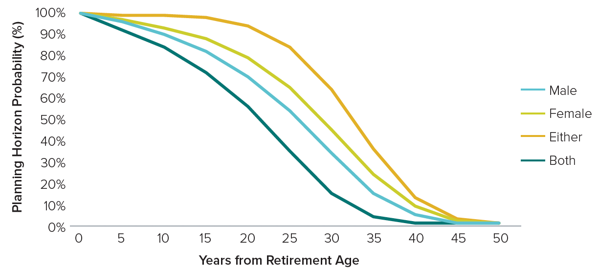
Source: Actuaries longevity illustrator, www.longevityillustrator.org/ as of 12/31/23
Redefining Risk for Retirement Income Strategies
It is commonly understood that the potential for future investment gains comes with some investment risk. Stemming from the pioneering work of Harry Markowitz (1952), who created the basic ideas of modern portfolio theory, portfolio volatility has been widely accepted as the most prominent risk. Volatility measures average risk; however, individual investors have varying concerns, time horizons, and goals. Protecting against losses may play a more dominant role for investors approaching retirement than managing volatility. In contrast, investors in retirement are generally most concerned with making their savings last while facing an unknown lifespan and rising prices. For these spending investors, we hypothesize that asset allocation is the most critical determinant of minimizing longevity risk or outliving one’s money. However, as investors in retirement are no longer accumulating assets, the asset allocation choice must be made in the context of minimizing longevity risk and protecting against losses to a level consistent with the investor’s risk tolerance.
A Summary of Retirement Income Research
The concept of a “safe” withdrawal rate in retirement is a subject of perennial interest, relevant to nearly everyone with retirement savings. Arguably the best-known guidance on this issue, the so-called “4% rule”, was popularized by William Bengen in 1994. Bengen examined historical U.S. market data along with a balanced portfolio of 50% stocks and 50% bonds and concluded that 4% was the highest sustainable spending rate during the worst thirty-year period of the study. More recently, Benz et al. (2021) from Morningstar stated that a reduction from 4% to 3.3% was more appropriate as a “safe” withdrawal rate under current market conditions for a balanced 50/50 portfolio.
Earlier works by David Blanchett (2007) complemented Bengen’s basic idea, concluding that fixed investment allocations outperformed declining equity glide paths popularized by target-date strategies. Dynamic allocations have also been examined more recently by Pfau and Kitces (2014), who found that an increasing equity glide path was more optimal in balancing protection against losses from a poor sequence of returns and maximizing portfolio longevity. Fan, Murray, and Pittman (2013) worked on modifying equity exposure concerning spending needs and shortfall risk (the risk of running out of money), confirming the notion that asset allocation has a significant impact on measures of success. Another classic article in the withdrawal literature was a study referred to as the “Trinity Study” by Cooley et al. (1998), which introduced the now ubiquitous statistic, the portfolio success rate. Our view is that since the portfolio success rate is closely tied to the investor’s objective of portfolio longevity, it is a more appropriate statistic to focus on than volatility alone for investors in retirement.
A primary factor in the relationship between portfolio success rates and asset allocation is the capital market assumptions used for the analysis. As Blanchett (2022) outlined, past research has used some simulated return paths based on actual historical time series or Monte Carlo variations. There have also been studies using measures of expected returns informed by valuation metrics (e.g., Pfau 2012 or Kitces 2009) or interest rates (e.g., Fink, Pfau, and Blanchett (2013)). We would refer the reader to Pfau (2017) for a detailed summary and history of other academic works on the topic.
Several common conclusions have emerged from this body of literature:
Higher stock allocations generally improve measures of success.
Factors that reduce growth rates, such as fees, taxes, or low capital market assumptions, diminish measures of success.
Flexible spending plans tend to provide better outcomes.
The gradual reduction in stock exposure as retirement nears, expressed in target-date-like strategies, can put portfolio longevity at risk. As we will demonstrate, considering risk metrics beyond volatility may significantly impact the optimal portfolio.
Searching for Optimal Allocations for Retirement Spending Plans
We used a standard withdrawal study to define an optimal asset allocation and compared it to other typical retirement spending portfolio solutions for our analysis. We assumed an initial distribution rate that increased with inflation each year after that from a portfolio of stocks and bonds. We simulated returns using conservative capital market assumptions and accounted for taxes and fees. We simulated 20-, 25-, and 30-year time horizons to span the range of expected planning horizons found in Figure 1.
Our core metrics were:
- A success rate is the percentage of simulated paths where all desired distributions are achieved.
- Real legacy wealth, or the wealth that remains, is defined as the average inflation-adjusted ending values as a percentage of the starting portfolio values. Additional details and assumptions of our methodology can be found in the Appendix.
FIGURE 2
Traditional success rates

FIGURE 3
Risk-optimized success rates for various distribution rates and equity allocations
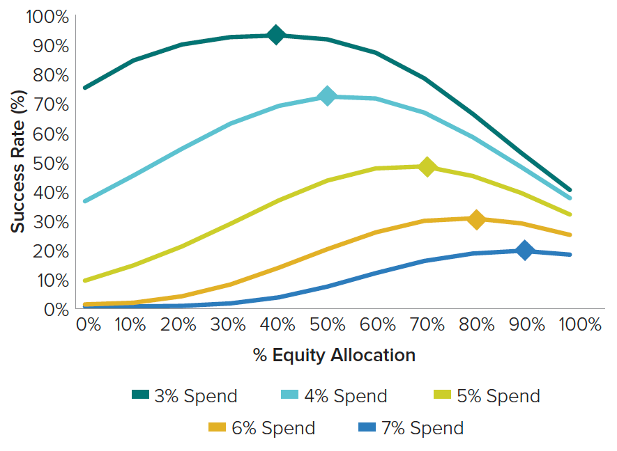
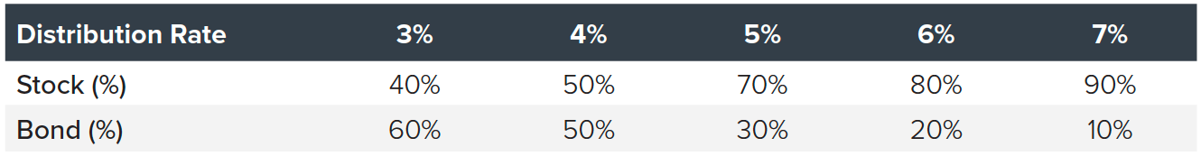
The rigidity with which spending was defined was a drawback of earlier studies on retirement income. The 4% rule is a good example – some investors might be more willing to accept a greater risk of failure to meet specific spending goals than others. Therefore, we believe it is necessary to define an optimal allocation for a desired distribution rate chosen by the investor instead of defining a single optimal distribution rate for a fixed allocation. In Figure 2 we vary the stock and bond allocation for each distribution rate and align with the conclusions of prior works that found increasing equity allocations improves measures of success for all starting distributions. However, we believe this result lacks suitability, as it does not account for any measure of risk tolerance. To incorporate risk, Figure 3 measures the success rate with the additional constraint that no annual return was worse than -20% for each path. We believe measuring risk tolerance in terms of portfolio losses practically matches how investors view longevity risk. We can observe an optimal asset allocation for each starting distribution rate by accounting for both portfolio longevity and portfolio losses. We call these fixed allocations Risk-Optimized Spending Strategies (ROSS) and use this as the primary strategy in our study. For conservative distribution rates, too much equity exposure is penalized by the loss constraint, while higher distribution rates require more equity exposure despite a greater risk of loss. The interaction and trade-off between this measure of success and risk tolerance allow us to identify optimal stock and bond allocations in Table 1 that we use in our study.
TABLE 1
Optimal stock and bond allocations for risk-optimized spending strategies (ROSS)
Comparison Strategy Descriptions
- 4% Rule – Constant Proportion (CP4)
The constant proportion strategy promotes a flat glide path through retirement. We use a 50% stock and 50% bond allocation here to proxy for the “4%-Rule” allocation. - Age-in-Bonds (AIB)
Age-in-bonds is a simplified case of a linear glide path that allocates an amount equal to the retiree’s age into bonds, with the balance of the exposure in stocks. - Target-Date Linear Glidepath (TD-LG)
Linear glide path strategies move a fixed portion of assets from stocks to bonds yearly. We use a standard target-date fund glide path for each planning horizon, starting with 60%, 55%, and 45% stock exposure, reducing the stock exposure by 2% each year with a minimum of 20% equity exposure.
Case Study Findings
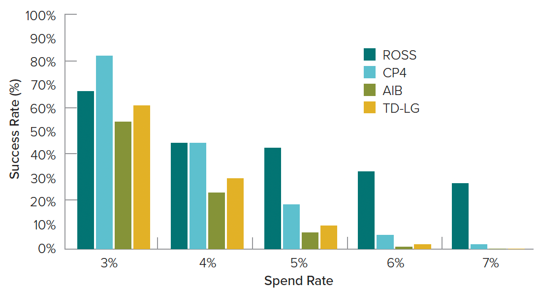
FIGURE 4
Traditional success rate by spend rate averaged across 20, 25, and 30-year spending horizons
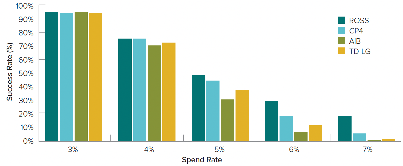 Source: Calculations by Horizon Investments
FIGURE 5
Average real legacy wealth as a percentage of starting wealth by spend rate across 20, 25, and 30-year spending horizons
 Source: Calculations by Horizon Investments
FIGURE 6
Traditional success rates averaged across spend rates of 3-7% by spending horizon
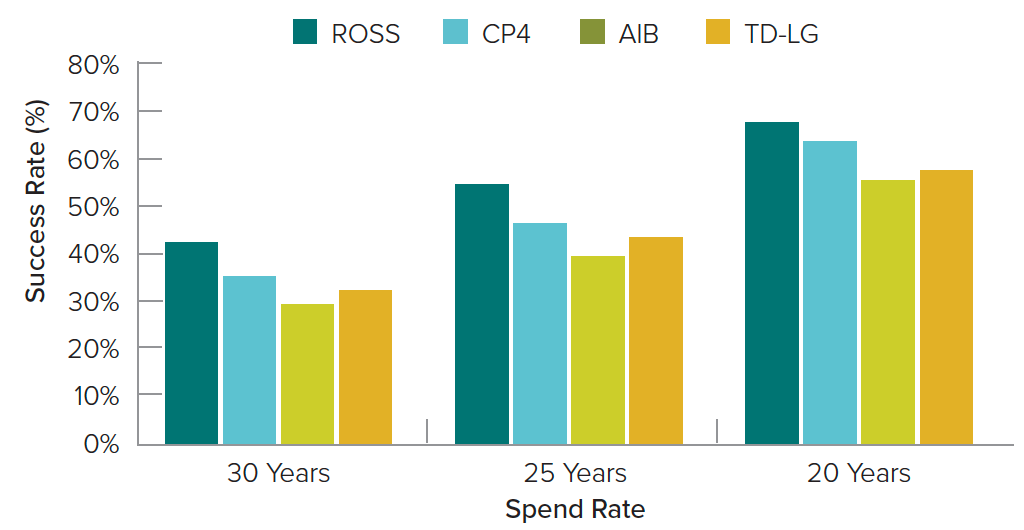 Source: Calculations by Horizon Investments
FIGURE 7
Average real legacy wealth as a percentage of starting wealth averaged across spend rates of 3-7% by spending horizon
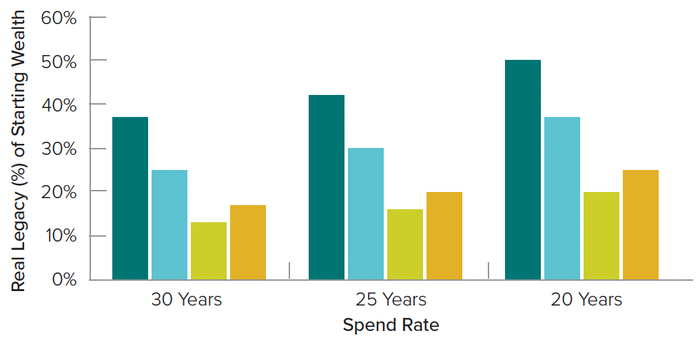 Source: Calculations by Horizon Investments